Numerical calculation of functional root

Functional root of function g(x) is function f(x), such that:

f(f(x)) = g(x)

General solution of this problem may be obtained via Abel's equation. here I will show a numeric approach, based on tailor series.

In general case, using Tailor series is complicated, but problem becomes much more simple, if g(0)=0. (or, in more general case, if there exists a such that g(a)=a. In this case, substitution g₁(x)=g(x+a)-a may be used)

More interesting thing is half-exponent: f(f(x))=e^x. Exponent does not intersects line y=x, so Taylor approach cannot be used. But if we consider complex x and y, intersection exists (furthermore, there are infinite number of intersections).

These points ma be found using Lambert's W function:

a0=-lambertw(-1)

Now let us shift to the point a₀ and calculate Taylor series at this point: g(x) = e^{x + a₀} - a₀

All derivatives of g(x) at 0 are equal to e^a₀. therefore let's use algorhytm b=ones(1,35)*a0; derivs35 k=f./factorial(1:length(f)); plot(abs(k(1:end-1)./k(2:end))) %from this plot we can see convergence radius that is about 1.3, which is close to complex part of a0. axis([0,35,0,2.5]) Therefore, this series can not be used for calculation of half-exponent at real axis. Newertheless, let's try x=linspace(0,1,100);y=polyval([fliplr(k),0],x-a0)+a0;yy=polyval([fliplr(k),0],y-a0)+a0; plot(x,real(yy),x,imag(yy),x,exp(x)) axis([0,1,-0.5,2]) 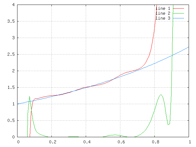This graph shows that convergence is really bad, but at interval [0.2..0.7] results are adequate. Looks like f(x) is significantly non-real for real arguments, though it may be result of bad convergence. Besides, equation exp(x)=x has other solutions. Maybe, they give better series? Let us try. a0=-lambertw(1,-1) a0 = 2.06227772959828 - 7.58863117847251i Radius is about b=ones(1,35)*a0; derivs35 k=f./factorial(1:length(f)); Radius is about 8.2, but |a0| is about 7.8. Alas, convergense still bad.

Files